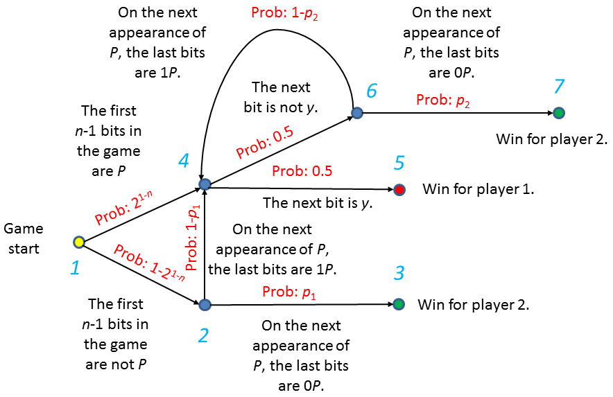
Figure 1: A state machine describing the game.
I first discovered this lovely game in a demonstration of math for kids at a local science museum. The demonstration came without any references, unfortunately, and for a while I wasn't able to track it down to its origins. A big thank-you goes to Yuping Luo for ultimately directing me to the right sources, because of which I can now give proper credit where it is due.
This game is known as "Penney Ante" or "Penney's Game". It was invented (fittingly enough) by Walter Penney in 1969. Its first publication was in October 1969, in the Journal of Recreational Mathematics. You can read about the game on Wikipedia and see an analysis of it in Concrete Mathematics, by Graham, Knuth and Patashnik.
What makes Penney's game so unintuitive is that it belongs to a class of games that are nontransitive. Let us say that the string chosen by each player is her strategy and that strategy A is a "good" strategy against strategy B if, when one player chooses A and another chooses B, the player who chose A has more than a 50% chance of winning the game. By saying that the game is nontransitive we mean that there are situations in which A is good against B, B is good against C, but C is good against A. For example, when n=4, a player choosing "1100" will win against a player choosing "0001" with probability 7/12, so "1100" is "good" against "0001". A player choosing "0110" will win against "1100", the previous winner, with the same probability, but "0001", the previous non-winner, turns out to still be a good strategy against the new winner, "0110", beating it 4/7 of the time.
This counters our intuition that if one strategy is good against another, it must be "better" than it in some global sense. In nontransitive games, that intuition does not hold. Though some strategies are "good" against others, there is no "best" strategy.
Because winning in this game is a probabilistic matter, this particular type of game is often described as a nontransitive probabilities game.
To understand where the peculiarities of Penney's game come from, note first that not all bit strings are equal in this game. As an example, consider a random string of 15 independent, uniformly-distributed bits. The probability that the string "00000000" appears in it is 9×2-9 but the probability that the equally-long string "00000001" appears in it is 1/32, almost twice as frequently. The reason for this is that while both strings have equal probability to appear at any given position, for "00000000" these various events have overlaps that reduce the total probability. The string "00000001", on the other hand, cannot appear more than once in a 15-bit string, so the various probabilities simply add up to create the total, with no need for any inclusion-exclusion in the calculation.
This property can be generalised. It was studied by A. D. Solov'ev in 1966 (three years before the invention of Penney's Game). Solov'ev was the first to note that the average "waiting time" (the expected number of generated bits before a particular bit string shows up) varies from bit-string to bit-string.
While (again, unintuitively) strategies in Penney's Game are not directly related to Solov'ev's waiting times (string A may be a "good" strategy against string B even if the average waiting time before its first appearance is greater than the average waiting time before B's first appearance), the probabilistic analysis of both relies on the same property: overlaps within the strings.
Here's another bit of counter-intuition this game conjures up:
Let us always extend the generation of random bits until Player One's bit-string appears. The probability of Player Two winning is the probability that in the output string (composed of everything the random bit generator generated throughout the extended game) Player Two's string also appears. However, note that this is not the same as the probability that Player Two's string appears in a random string that terminates with Player One's string. The difference is that in the actual game we also require that Player One's string never appeared previously.
For example, the probability for a 9-bit string that terminates with "00000000" to also contain "10000000" is 50%, but if in the actual game Player One chose "00000000" and Player Two chose "10000000", and if the extended game terminated after 9 bits, then Player Two is guaranteed to have won. (The choice 0n is undoubtedly the worst choice Player One can make in this game. If the first n bits are all zeroes, Player One wins, but otherwise Player Two is guaranteed to win if she chooses 10n-1. Because Player One has a probability of 2-n of winning after exactly n bits regardless of her choice of string, the choice 0n, which attains this winning probability in total, guarantees the worst possible winning probability for Player One.)
Taking care to rely on rigorous analysis rather than intuition, however, let us proceed to answer the questions, beginning with questions 1 and 2.
The cases n=1 and n=2 are easy to analyse exhaustively. In both cases, the optimal strategies yield equal win probabilities for both players. We therefore restrict ourselves to the case n≥3.
Let the string chosen by Player One be "Py", where P is a bit-string of length n-1 and y is a bit. We assume that this string is neither 0n nor 1n, which are cases already analysed above. We will show that Player Two can always win with probability at least (2 - 21-n)/3, by choosing either "0P" or "1P" as her chosen string. In particular, for n≥3, Player Two can guarantee a win probability in excess of 50%.
To show this, let us consider the game in progress, pausing it at certain interesting points. Specifically, Figure 1 shows a state machine describing the probabilities governing a game where Player One chose "Py" and Player Two chose "0P". The various states depict the game at game start, after n-1 bits have been generated, and whenever the last string of bits generated was "P", "P0" or "P1". We note that given our choice of strategies for the two players, these states cover, in particular, all terminal states.
To be able to name the transition probabilities, let p1 be the probability that a random string of length at least n bits that terminates in P and has no prior appearances of P in it will have "0P" as its n-bit suffix, and let p2 be the probability that a random string of length at least n bits that starts with P followed by the negation of y, that terminates in P and that has no other appearances of P in it will have "0P" as its n-bit suffix. (By "random string" we mean, a string randomly generated by the process described in the riddle, whose termination criterion is the n-1 bit string P.)
The winning probabilities can be calculated easily from the diagram as functions of p1 and p2. The only loop in the diagram is at the node numbered "4". Once reaching node "4", Player 1 may win immediately at node "5" with probability 0.5, Player Two may win at node "7" with probability 0.5p2, or the game may return to "4" and another round with the same conditional probabilities will repeat. In total, this means that once reaching "4" the ratio of Player One to Player Two wins is the ratio 0.5 to 0.5p2, so the total win probability for Player Two from node "4" is p2/(1+p2). The rest of the diagram contains no loops and is straightforward to analyse.
In total, excluding, once again, the cases 0n and 1n for Player One, which have already been dealt with, the probability of Player Two winning by choosing "0P" over Player One's "Py" is
| W0 = (1-21-n)p1 + ((1-21-n)(1-p1)+21-n) × p2 / (1+p2) | (1) |
Player Two's winning probability if she chooses "1P" instead of "0P" can be calculated in the same way. All one needs is to replace every appearance of p1 by 1-p1 and every appearance of p2 by 1-p2. The result, once simplified slightly, is this:
| W1 = (1-21-n)(1-p1) + ((1-21-n)p1+21-n) × (1-p2) / (2-p2) | (2) |
To show that at least one of these strategies has a high win probability, note that for any given p2, W0 is a linear function, monotone increasing in p1, while W1 is a linear function, monotone decreasing in p1. The worst winning probability for a Player Two choosing between one of these two strategies will therefore occur when p1 is set exactly so that W0=W1. This happens when
| 3×(1-21-n)×(p1-½) = (1+21-n)×(½-p2) | (3) |
Substituting Eq. (3) back into Eqs. (1) and (2), we get that Player Two can always guarantee a winning probability of at least (2 - 21-n)/3, as desired.
Q.E.D.
Note that asymptotically, this gives a lower bound of 2/3 winning probability for Player Two, no matter what Player One chooses.
To answer question 3, we will calculate the exact probabilities of winning in every case. These probabilities were first discovered by John Horton Conway (credit to Conway was given by Martin Gardner in his October 1974 Mathematical Recreations).
Let us define the function w(S), for any set of strings, S, to be the sum, over all strings s in S, of 2-|s|. In particular, if we take Player One's string to be a and Player Two's string to be b, and if we define A to be the set of all strings the can be generated during the course of the game that result in Player One winning (i.e., all strings that terminate in a but have no other appearances of a or b in them) and if we further define B to be the set of all strings that can be generated during the course of the game that result in Player Two winning, then w(A) is the probability of Player One winning and w(B) is the probability of Player Two winning.
To calculate these, let us introduce a further set, N, which is the set of strings that can be produced while the game is still in progress (i.e., the set of strings that include neither appearances of a nor of b).
Furthermore, let us introduce the function [u:v], where u and v are strings of length n, as the sum of 2-k over all k values in the range 0≤k<n satisfying that the last n-k bits of u are equal to the first n-k bits of v.
Now, supposing we take every element in N and append to it a. Certainly, this is a string of bits that represents a game already terminated, but at what round was it terminated, and who won? It may be that it only terminated with the appearance of the appended a, but if the first n-k bits of a happen to coincide with the last n-k bits of either a or b, then this game could have ended k steps earlier, if the k-length suffix of the original string happened to coincide with the remainder. So, this string can equally be thought of as an element of A (or B) to which the k-length suffix of a was appended.
Figure 2 demonstrates this with an example.
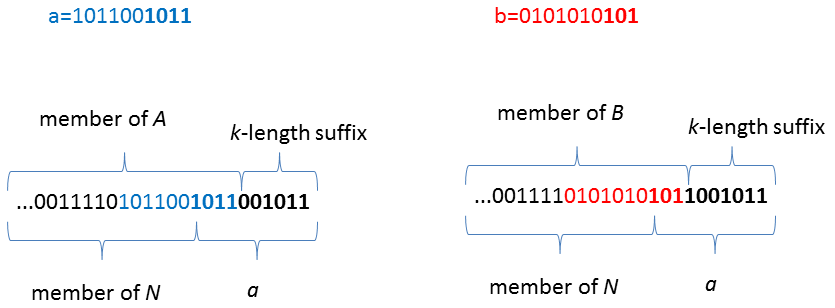
Calculating w over this new string set clearly yields w(N)×2-n, because each of the original strings from N was increased in length by n bits. However, due to the rationale given above, the same set of strings can be produced by strings from A or B to which an appropriate suffix has been appended. These suffices are precisely those counted by the [a:a] and [b:a] functions, and the weight that one needs to give to them are also as calculated by these functions. In total, one arrives at the following equation:
| w(N)×2-n = w(A)[a:a] + w(B)[b:a] | (4) |
(For those wanting complete rigour in the analysis, we remark that w(A) and w(B) are known not to diverge, because they are the probabilities of winning, whereas w(N) is known not to diverge simply due to this equation, which presents it as a finite linear combination of probabilities.)
Repeating the same process, but appending to elements of N copies of b this time, instead of a, we reach the equation
| w(N)×2-n = w(A)[a:b] + w(B)[b:b] | (5) |
As the left hand side of both (4) and (5) is equal, the right hand sides must also equal each other. This leads us to the equation
| w(B)/w(A) = ([a:a]-[a:b]) / ([b:b]-[b:a]) | (6) |
this equation giving exact winning odds for the players.
For n>3, the optimal strategy for Player One turns out to be choosing the string 10n-311. We will not prove its optimality, but will, rather, show that asymptotically it gives the second player 2:1 winning odds, which is exactly the asymptotic lower bound on the winning odds of the second player given any choice by Player One, as calculated in the answer to question 2.
To see this, let us bound (or calculate) the elements of equation (6), given the chosen a and any b.
First, we can calculate [a:a] exactly.
| [a:a] = 1 + 21-n | (7) |
Next, we have
| [b:b] ≥ 1 | (8) |
because the string must at least equal itself.
Let us now consider [b:a]. For how many separate k values can the last n-k values of b coincide with the first n-k values of a? Suppose we found one such k, then the suffix of b must be "1000..." (or, if it's of length n-1, "100...001"). This excludes all similar prefixes for other values of k. The only pair of k's that may coexist are k=1 (the suffix of length n-1) and k=n-1 (the suffix of length 1). As it is not possible for k to be zero due to a≠b, this bounds [b:a] at
| [b:a] ≤ 0.5+21-n | (9) |
Putting all this together, we get
| w(B)/w(A) = ([a:a]-[a:b]) / ([b:b]-[b:a]) ≤ [a:a] / ([b:b]-[b:a]) ≤ [a:a] / (0.5-21-n) ≤ (1 + 21-n) / (0.5-21-n) | (10) |
which, asymptotically, is the same 2:1 ratio that was reached in the answer to question 2.
Q.E.D.
Beyond what was asked in the riddle:
One can perform the same kind of analysis, starting from equation (6), to reach lower bounds for the winning probability as a function of [b:a]. This analysis proves that, given this particular choice of a, only a b value for which [b:a]≥0.5 can reach winning probabilities such as those found in our answer to question 2. This, in turn, narrows b to be one of the two values from the strategy given in the answer to question 2, which, in turn, allows us to calculate the optimum exactly for every n: if Player One plays "10...011", Player Two's best response is to play "010...01", reaching winning odds of (2n-1+1):(2n-2+1).
In 1992, J. A. Csirik proved that for any n>3, this is, indeed, the optimal strategy for Player One.
Totalling all the references given here, it seems that this problem remained open for 23 years, from 1969 to 1992 (more, if you count Solov'ev's work) after having been considered by some of the very greats. An illustrious history, for such a simple-looking puzzle!